Murder and relative frequency: Exploring linguistic data

This very long post is an exercise for some classes that I’m teaching at the EUROLAN “summer school” on biomedical natural language processing.  I put it here to give you a taste of what a computational linguist actually does all day; if you just want to see the English notes, scroll down to the bottom.

So, you’re a linguist.  Or, you’re a software engineer who’s been told to build a system that does something with language.  You’re a researcher in adolescent reproductive health, and you want to find out why teenaged mothers have implanted birth control devices removed.  Maybe you’re an artificial intelligence researcher who figures that using language is the most intelligent thing that we do, and so you want to explore what kinds of computer models would be sufficient to do that—artificially, of course. You’re a biologist who wants to build a database of genes involved in emphysema, or you could be a sociologist who wants to see how sexism is manifested in newspaper articles, and you want to know if that has changed between when we started publishing newspapers in America (the early 1700s) and the passing of the Equal Rights Amendment through both houses of Congress in 1972.  Maybe you’re a crime analyst, and you realize that it would be useful to have a computer program that could read through what the police wrote in tens of thousands of reports of car thefts.  (I don’t make this stuff up!)  Either way, you need some written data to do your thing, and you need a lot of it.  The good thing about having a lot of it is that you might have a valid sample; the bad thing about having a lot of it is that there’s no way in hell that you can answer your questions just by reading it all.  Computational linguistics to the rescue.

Computational linguistics can be described as building models of language that can be turned into a computer program.  Some of the advantages of this come from the fact that it forces you to be incredibly specific about what your model is built of.  Some of the advantages of this come from the fact that you can test that model on big bodies of data.  To do that, you need to get one of those big bodies of data.  Problem is, though: you can’t read it all.  You could pull out samples of it, but Zipf’s Law means that your sample, as valid as it maybe be, is mostly going to just tell you about the frequent stuff.  So, you need a way to learn about your data’s characteristics that you can apply on a large scale; a way to learn about your data that will tell you about the variety of things that happen in it without falling into the trap of only finding the frequent stuff.

That means that you actually need not just “a way,” but a variety of ways.  In today’s hands-on session, we’ll look at some of those.  We’ll focus on (relatively) simple ways, but bear in mind that all of them can be made more sophisticated—at the cost of being more complex to write the programs for, but with the benefit of being more powerful in terms of what you can do with them.  But, more on that another time.

---

As we mentioned above, one of the advantages of this kind of approach to language is that it can deal with large amounts of linguistic data.  Here’s the thing, though: in order to do that, you actually have to have a lot of data in your hands.  This turns out to be the most common cause of failed projects in computational linguistics—relying on being able to get data that it turns out you can’t get your hands on.  (To get your hands on something explained in the English notes below.)  You think I’m exaggerating about that?  Read this.

The first thing that you do is find out how much data you have.  Recall that we do this stuff in order to deal with big bodies of data, so you want to ensure that you do, in fact, have a lot of it—or, if you don’t, in fact, have a lot of it, you want to learn that fact immediately, so that you can do something about it.  How do you do this?

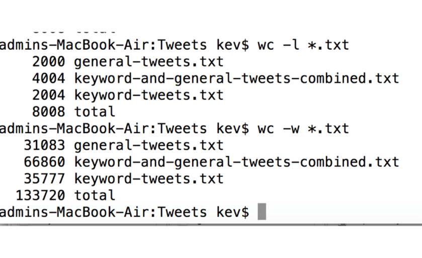
The most common thing that a computational linguist would use is a computer that has the UNIX operating system on it.  Twenty years ago, that meant computers in labs; today, it means those, plus all Macintosh computers.  These let you run a command called wc.  wc stands for “word count.”  The program splits your data wherever it sees a space, and counts how many things that results in.  Here’s how you use wc:

Let’s suppose that you have as much data as you need.  (How much data do you need?  That’s hard to answer without knowing what you’re going to do with it—and a lot of other things.)  How much you’re actually going to get: that depends on how much you can afford.  A corpus (linguistic data) construction project determines how much data it’s going to make by starting with the amount of funding that it’s been able to get, dividing that amount by the cost per unit of data, and that’s how much you’re going to get—max.  But, yeah—you’ve managed to get your hands on some data.  What’s the first thing to do when you sit down at your desk on that first beautiful Monday morning?

Wondering why I talk about tweets so often?  Read this on the subject of natural language processing, social media data, and suicide.

Looks easy, right?  wc is the name of the program. *.txt means “do this to every file whose name ends with .txt.  wc –w tells you the number of words, while wc –l tells you the number of lines of data in the files.  (If lines are meaningful, that can tell you something about larger units in the data—in the case of this data, it’s tweets, and the files contain one tweet per line, so counting the lines told me how many tweets I had.) The number is the number of words/lines in those files, followed by the total for all files.  (Using a Windows machine?  Try this web page for some possible ways to do it.)  Don’t feel bad if you messed it up, though–I did.  My totals are wrong here, because I messed something up by using *.txt instead of specifying the names of the files more carefully.  Can you tell what I did wrong?  Hint: my mistake caused a seriously large over-count of the number of words.

…and that brings us to your first exercise:

You can download the CRAFT corpus of journal articles about mouse genomics here.  For information about the corpus, see this article from Nancy Ide’s recent book on linguistic annotation.

1. Find out how much data you have in the test file test.single.file.txt that you downloaded from the GitHub repository for these exercises. Do the same for the text files in the CRAFT corpus.

So, now you know how much data you have.  (Well, you have a guess—we’ll see later why this isn’t the end of the story.)  Now you ask a question: is this enough?  If it is: keep going.  If it isn’t: do something about it.

---

The second thing that you do is find out what the basic distributional properties of your data are.  One of the themes of this blog is the implications of the statistical properties of language.  That implies that language has particular statistical properties.  One of the very important of those properties is that large samples of language follow Zipf’s Law: a very small number of words occur very frequently; the vast majority of words in a language almost never occur—but, they do occur, and that has implications for many things, ranging from your approach to learning vocabulary in a second language to the kinds of statistical models that you can use in computational linguistics.  So, it probably won’t surprise you that a useful thing to do first with your data is to see to what extent it does—or doesn’t—behave as Zipf’s Law would suggest.

One way to do this is to build a particular kind of graph.  We’ve seen it many times on this blog, but have never gone through the mechanics of how to build it.

Another thing that you can do is figure out how closely it fits Zipf’s Law.  We’ll talk in a bit about what “fit” means in this context—for now, let’s look at the formula that expresses Zipf’s Law.

Zipf’s Law is about the relationship between frequency and rank, so let’s start by defining what those mean.

Frequency is a count of how often something occurs, normalized in some way–for example, how often per million words of text.  Think of it this way: if you ask me how often I eat, and I say three times, what does that mean, exactly?  If it means three times over the course of my life, then my life will be pretty damn short.  On the other hand, if it means three times per day, then I will probably live at least until the beginning of the zombie apocalypse, if the man-eating rabbits don’t get me first.  We’ll come back to the question of what-are-word-counts-relative-to later.

Rank refers to your position in a list, where that list is ordered by some principle.  Think about the waiting line for a subway ticket window.  In Paris, that line is ordered by the principle of who got there first.  Compare that to the order of soldiers in line in a formation.  That line is ordered, too—by height.  Compare that to the horde of people trying to fight their way out of a burning building—that probably isn’t ordered at all.

Suppose that we count how many times each word occurs in some body of data.  Then we’ll order the list of those words by frequency.  Suppose that we count a bunch of articles about mouse genomics.  (We care about genes, in part, because many diseases involve genes in some way; we care about a mouse’s genes because we can’t experiment on humans with diseases, but we can experiment on mice with diseases, and genetically, mice are pretty much like humans.)  …and that brings us to your second exercise.

2.  Write code to count the number of occurrences of each individual word in the text files whose contents you counted in the first exercise. See below for what your results should look like.

Suppose that we get the following counts:

bone 100
density 90
the 100000
thickness 1
and 10000
mouse 500
vasculature 1
parenchyma 1

(In the test file, the word one occurs 1 time, the word two occurs 2 times, and the word five occurs 5 times; your counts should reflect that.)

Now let’s put those in some sort of order.  We’ll base our order on this principle: bigger counts first.  That gives us this:

the 100000
and 10000
mouse 500
bone 100
density 90
thickness 1
vasculature 1
parenchyma 1

Pretty simple so far.  Not as simple as it might seem, though—notice that three of those words occur the same number of times.  If we’re ordering words by count, then what do you do with ties?  But, conceptually, it’s easy enough.  Mostly.  Seems like a good time for your third exercise:

3.  Order the words whose frequently you counted in the second exercise, with bigger numbers first.

That seems simple too, right?  Actually, there are a number of ways to screw it up: using alphabetical order, primarily, which will give you the order 1, 10, 100, 1000, 2, 20, etc.  You need to use the right comparator–figure out what it is in whatever language you’ve chosen to use.

So, now we have a list of words, and we’ve ordered it by count.  To see if this sample follows Zipf’s Law, we need one more number: we need each word’s rank.  Recall the definition of rank: your position in that list.  So, your fourth exercise:

4.  Figure out a way to know the rank of each word in your list.

Take a moment to look at what the frequent words are—they should “make sense” in terms of what you expect.  Are they what you would expect?  For example, if you think that you’re dealing with normal English, you should expect that words like the and and will be way up towards the top.  On the other hand, if you think that you’re looking at a bunch of weather reports, then maybe you’ll expect to see F way up towards the top.  Either way: if what you see doesn’t make sense, then you should figure out why.  (Maybe the person you asked for the data didn’t give you what you asked for.  Maybe you’re actually looking at image files.  Mistakes happen—they’re a fact of life.  I make them, you make them, the smartest people in the world make them.  You just need to find them, that’s all.)

…and now we’re ready to get our first graphical look at our data!

Visualizing patterns in your data can be much more revealing than looking at tables of numbers—for a statistician, it’s the beginning step in any analysis.  To do that, we need to know the frequency and the rank of each word.  When we have data that is ordered in some way such that we can think of one value as greater than the preceding one, a kind of graph called a line graph makes sense.  (Line graphs don’t always make sense—find some examples.)

We’ll put the frequency of each word on the y (vertical) axis, and the rank of each word on the x x (horizontal) axis.  (Why are they called that?  I have no idea.  Someone?)  Each point on that graph is a word; the position of that point on the y axis corresponds to its frequency, and the position of that point on the x axis refers to its rank.  (You figured out the frequency in Exercise X, and the rank in Exercise Y.)  Here’s a single word:

Sorry, I didn’t get the graph finished!

Add every word, and you have a bunch of points.  Add enough words, and you get a line.  Here’s what that looks like for our data: …nor this one!

…which brings us to your next exercise:

5.  Graph your results as described above.

Now let’s think about what that graph is showing us.  A very small number of words very frequent, a large number of words very rare.

Dan Tufis tells me that one cool use of Zipf’s Law was testing whether or not the Voynich Manuscript contains actual language.

Zipf’s Law is logarithmic-ish, so it would make sense to look at this data by graphing the log of those frequencies and ranks, rather than the actual frequencies and ranks.  The advantage to doing this is that we know exactly what the line will look like if the relationship is really logartithmic: the line will be straight.  Lines that aren’t straight at all reflect a relationship that just plain isn’t algorithmic–a data set that isn’t Zipfian, and that we should therefore be a bit suspicious about.  (For example, a linguistic data set could fail to show a Zipfian distribution because it isn ‘t sufficiently large–a problem in natural language processing, because then you suffer from the curse of sparse data, while not receiving the blessing of having some things occur frequently enough for you to be able to build good rules–or statistical models–for them.)  Lines that are straight in the middle, but not at the top and bottom, reflect data that mostly conforms to the prediction of Zipf’s Law, but doesn’t conform to it well for the extreme ranks (i.e. the very high ranks, and the very low ranks).  That’s actually pretty common, and some of the later modifications to Zipf’s Law were made to try to account for that fact.  And that brings us to your next exercise:

6.  Graph your results on a log scale.

---

The third thing to do is to look at the relative frequencies of things in your data.  We need to talk about frequency a bit more.  The point of counting anything is to compare it to something else.  For different data set sizes, you need to have frequencies that are relative to the same number.  Maybe.  So, let’s do that: we’ll compare these number to some reference corpus.  (We’ll talk about picking a reference corpus in a couple minutes.)  This means doing all of the calculations that you did above to find frequencies for another corpus, and then taking the ratios of the frequencies of each word in your corpus to the same word in the other corpus.  (What are you going to do about words that never occur in the other corpus?  If they only occur once in either corpus, you may want to discard them–for example, they may just be spelling errors.  If they occur more than once in one corpus, but never in the other, then you should use a smoothing technique.)

So, what can you find out by comparing frequencies?  Obviously, you can find rank with respect to other words in your data—that’s where we started.  But, you can learn a bunch of things by looking at frequencies relative to other data sets.  In fact, that’s where you first start to get some insight into the contents of your data, as opposed to its sizes/counts.  Something beyond raw numbers, getting into contents.

Relative to the frequencies in what other data??  The questions that you’re asking by doing this analysis are different depending on what that other datas.  Imagine mouse genomics versus newspaper articles—you’re probably learning about scientific language, more than mouse genomics.  Imagine mouse genomics against a random sample of scientific journal articles—now you’re actually probably learning something about mice.  Now imagine mouse genomics versus random articles about mice—now you’re probably learning something about genomics.  None of those are mouse genomics, which is what you thought you were finding out about.  And that takes you to the next exercise, which is to think about this question:

7.  Is this actually an important problem, where “important” means that I need to solve it if I’m going to be able to believe my results?  If so: why is it important?  If not: why is it not important?

So, now let’s calculate the relative frequencies, and see what they tell us about our data set.  But, before we act: let’s think.

Why would you expect relative frequencies to tell you anything of interest about your collection of data?  Because relative frequencies help you separate the things that are different between the two corpora from the things that are similar in the two corpora, and as we’ve discussed before, most of what we’re interested in in science (and in life, actually) is how things are different from each other.  (Remember that the “null hypothesis” is that everything is the same.)  But, how does relative frequency tell you what’s similar and what’s different?

Before we run this little experiment, though, let’s think first about what things will probably have similar relative frequencies in our two sets of data, and then we’ll see what that means in terms of the output of the calculations.  (Thinking about this before we do the calculations will help to ensure that we do them correctly.)  Would we expect the frequencies of rare words—collusion, liar, bully—to be similar?  No—those are either going to be zero, or not, and in either case, they don’t really tell us much.  (Spelling errors are about that rare, and they don’t tell us that much about the contents of our data set, either, other than that the data isn’t perfect, which we already knew, ‘cause I’ve told you that a million times this week already: no data is perfect.

The words that we would expect to have similar frequencies in the two corpora are the words that express what we might think of as “grammatical” functions: the, and, to, of.  Unless you have very unusual data in one of those data sets, the distribution of that kind of word is about the same in any kind of data in a given language.  (When it does differ, it’s sometimes very revealing, and in some kinds of clinical texts, it can vary quite a bit.  Most of the time, though, it doesn’t.)  (You can find some fascinating experimental findings about the distributions of those words in studies of mental illness in James Pennebaker’s book The secret life of pronouns.) When you have frequencies that are very close to each other, then the value of the relative frequency is close to 1.  For example:

Frequency of word xyz in data set A is 100 words per million; frequency of word xyz in data set B is 97 words per million; relative frequency is 100/97 = 1.03. 

Frequency of word abc in data set A is 97 words per million; frequency of word abc in data set B is 100 words per million; relative frequency is 97/100 = 0.97. 

So:

8.  Calculate the relative frequencies.

9.  What kinds of things do you see at the top, and what kinds of things do you see at the bottom?

10.  Re-calculate them with small, medium, and large smoothing values.

11.  Re-calculate them with different reference corpora.

So: words with similar frequencies in the two data sets will have a frequency close to 1.  In contrast, words with different frequencies in the two sets will have relative frequencies that are far from 1.  That raises a question: far from 1 by being much bigger than 1, or far from 1 in by being much smaller than 1?  The answer: it depends on which corpus they occur in more often.

If a word occurs much more often in the data set whose frequency goes on the top half (numerator) of the fraction, then the relative frequency will be much larger than 1.  (By convention, we usually put our data set in the numerator and the reference data set in the denominator, but it doesn’t matter.  When we do it this way, larger numbers tell us about our data set, which just seems to feel right to people.  Like I said: it doesn’t actually matter.)  On the other hand, if the word occurs much more often in the data set whose frequency goes on the bottom half (denominator) of the fraction, then the relative frequency will be much smaller than 1.

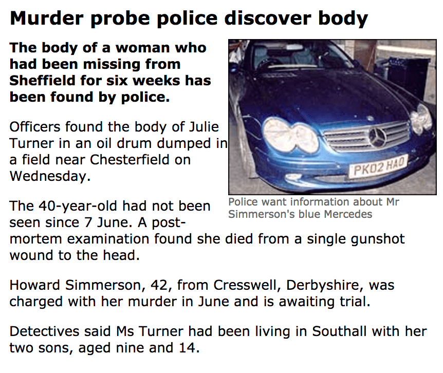
You think that I’m making too much of relative frequencies?  They were used to help solve this murder in England 10 years ago.  The linguist involved in the case used various corpus search tools to compare some things that appeared in text messages from the missing woman’s phone with some things that her boyfriend said in an interview with police, and compared their relative frequencies with a number of corpora.  The results convinced the police that they should turn what had been a missing persons case into a murder investigation and focus on the boyfriend as their suspect.  He turned out to have killed the victim and stuffed her in an oil drum.  You can read the details of the analysis done by the linguist in question, John Olsson, in his book Wordcrime: Solving crime through forensic linguistics.

---

Let’s look at some examples.  Suppose that data set A is a bunch of journal articles about mouse genomics, while data set B is a set of newspaper articles about the Trump administration.  In that case, we would expect the word gene to be much more common—i.e., to have a larger frequency—in the set of articles about mouse genomics than in the set of articles about the Trump administration.  On the other hand, we would expect the word liar to be much more common—i.e., to have a much higher frequency in the set of articles about the Trump administration.  If we suppose that the word gene occurs in the mouse genomics articles 100 times per million words, but only one 1 time per million words in the set of articles about the Trump administration, while the word liar occurs 100 times per million words in the set of articles about the Trump administration, but only 1 time per million words in the set of mouse genomics articles, then we have the following relative frequencies:

Gene: mouse genomics frequency = 100/million, Trump administration = 1/million.

Relative frequency = 100/1 = 100.0.

Liar: mouse genomics frequency = 1/million, Trump administration = 100/million.

Relative frequency = 1/100 = 0.001. 

So, being far from a value of 1 means that you are more characteristic of one data set than the other; in a sense, it doesn’t matter whether you look at the big numbers, or the little ones.  By convention, we’ll put the data set that we care about on the top of the fraction (in the numerator), so to see which words reflect the contents of our corpus, we’ll look for the big numbers.  (That’s mostly arbitrary, but there are probably also some repercussions related to looking at numbers much larger than 0 versus numbers that are much smaller than 0 from the point of view of how computer memory works.  Can someone enlighten the rest of us as to whether or not that’s an issue?) …and this brings us to your next exercise:

11. Use the frequencies that we calculated earlier to calculate the relative frequencies for the words in your data set, as compared to some reference data of your choice. What are the top-10 over-represented words in your data, and what do they tell you?  Some sources of reference data: you can find Nancy Ide’s Manually Annotated Sub-Corpus of the Open American National Corpus here (text data only, which is all that you need for these exercises).

12.  Is there some significance to the words that are over-represented in the other data set, as compared to yours?  Significant in the sense of telling you something about your data?

---

Now, there’s a big question that we’ve ignored up to this point: What should you actually be counting here??  “Trivial” preprocessing matters more than might be obvious.  A “small” step that can matter a lot in your calculations of frequency can matter a lot here–I’ve seen people do this where they calculated the frequency of words relative to the number of tokens in their data rather than relative to the number of words in their data.  That is: they counted the frequency of words relative to words plus all punctuation marks, which is almost certainly not what you want to do.  And, of course, tokenization looks simple, but it isn’t–see Noa’s paper on this, and every paper that every looked at tokenization specifically, and every machine learning paper that ever mentioned it in passing without really thinking about how much difference it made in their results.  Compare the magnitude of the differences due to preprocessing in Noa’s paper with the magnitude of the differences in a typical ACL paper.  This should make your blood run cold—but, more on that another time.

Now, so far we’ve been looking at things that you could think of as …  I don’t know…  general statistics about the entire document collection.  No matter which of the many reasons that I gave at the top of this post is driving you to tear your hair out trying to get your computer to do this stuff, the things that we’ve been doing will probably be useful to you.  But: you probably have some very specific sorts of questions that are going to be important to what you, personally, do—and that won’t get answered by the general statistical characterization that we’ve been doing up to this point.  For example: most of you are involved in some way in trying to write programs that find information in text.

Information extraction—finding information in written texts, the subject of Pierre’s lecture on Friday—tends to have problems with some pretty specific things.  Whether people are working with medical records, journal articles about mouse genomics, or reports of car thefts, they tend to run into trouble with the same three things:

1. Pronouns
2. Conjunctions
3. Negation

…and that brings us to your next exercise:

 13.  Write code to calculate the frequencies of one of these things, and compare their frequencies to some reference corpus or corpora.

There are lots of ways to count these, some of which are more efficient than others.  I generally prefer clarity over efficiency, so in the code that I give you, you’ll see a slow way to do it, but hopefully it will be clear to you what I’m doing (or trying to do).  Try it on the CRAFT corpus data on the GitHub page—I would be super-interested in seeing how your results differ from the results reported in this paper (and super-shocked if they don’t differ).

At about this point in these exercises, you should be asking yourself these questions:

a.  How long did it take me to use this for the easy-to-use corpora that Kevin put together for the didactic purposes?

b.  How much time to I have left to write my master’s thesis/doctoral dissertation/article/grant proposal?

If you conclude that you are not going to have enough time to do even a basic analysis of your data before you have to dive into your experiments, you should think very hard about going to your supervisor and explaining why you need to renegotiate what you’re trying to do.

---

Beyond these basic distributional questions, there are some other relatively straightforward things that you can do to understand your data a bit better.  For starters: think about it in terms of terminology, especially if you’re dealing with biomedical or other scientific or technical data.  To wit…

Consider thinking about the contents of your corpus as being built from a set of terms.  By definition, “terminology” is the set of words and phrases that are specific to a particular subject, as opposed to the language in general.  That doesn’t mean that they’re not part of the language in general—it means that they form a set that you can think of as a sort of definition of what the domain is about.  For you, this means that if your data is coherent in some way with respect to its topic (often the case in the biomedical domain), and if you have access to terminology extraction software, then you can run your data through the terminology extraction software.  As you might guess, this does something similar to the relative frequency stuff that we worked our way through earlier in this exercise; the difference(s) are that terminology extraction software usually has more sophisticated algorithms.  (The usual trade-off between high performance and being able to understand what the hell you just did.)  Here’s the results of running the directions for these exercises through one terminology extraction tool, found at http://keywordextraction.net/keyword-extractor:

1. terminology extraction software
2. natural language processing
3. computational linguistics
4. statistical properties
5. mouse genomics

This tool requires you to specify how many terms you want, and has a default setting of five.  Of those five, I’d say that 2-4 are pretty accurate representations of what these exercises are about.  5 is certainly something that I talk about a lot, but it’s hard to say that mouse genomics is what this is about, per se.  1 clearly is not what this little essay is about—tells you something about the code’s balance between being over-represented relative to a reference (clearly terminology extraction software would be absent in almost any body of textual data in the world) and not being cautious with respect to very low-frequency items (remember that we had that on our list of things to think about when doing our relative-frequency calculations).

Here are the results from another terminology extraction tool, Termine, from the National Centre for Text Mining in the UK.  (This is the terminology extraction tool that I use myself.)  Note that Termine gives you a lot more information than the other tool did—we get the scores that are the source of the ranking, and we can use that to make intelligent choices about how far down the list to go when we’re analyzing the data.  (I have 7 terms in the example because I wanted the top 5 to compare with the other tool’s top 5, and here we have 3 terms tied for 5^th place.)  Looking at the results, we can see the hints of some of the processing decisions that the authors made: notice that linguistics has become linguistic, and genomics has become genomic—this is a pretty good clue that Termine does some work to try to treat singulars and plurals as the same.  (Look at the list below of similar decisions that will affect your results with the relative frequency calculations, too.)  It’s also reasonable to guess that Termine does more to address the rare-words issue than the other tool does, since although Termine also found terminology extraction software, it ranked it third, rather than first.  Overall, Termine is my go-to tool for this kind of thing, and it’s especially good for biomedical journal articles, which a number of you are working on, as it uses some processing tools that are specialized for scientific publications.

Now, we’ve put together this little set of exercises on linguistic data exploration on the assumption that we were working with words, without ever (1) defining what we mean by “word,” or (2) thinking about the possibility of looking at other things besides words.  We haven’t talked about smoothing our models, or about dealing with hapax legomena–like, say, measurements, which about in both scientific and medical texts, and which are essentially worthless (or even harmful) to us, but which might be very useful if we considered any number as an abstract instance of a number, while ignoring the actual value itself.  Here is a short list, off the top of my head, of things that you need to think about in order to take this kind of question into account:

1. Tokenization choices
2. Capitalization normalization, or not
3. How you handle low-frequency and zero-frequency words (how can a word have a frequency of 0 in this case?)
4. Mis-plessings
5. Numbers
6. “Named entities” (what might be helped/hurt if you lumped together all mentions of locations? All mentions of people?  All mentions of medications/genes/species/diseases/…?)
7. Bigrams instead of words
8. Collocations instead of bigrams

…and that takes us to your last exercise:

14.  Think of something that should be added to the preceding list.  In the Comments section, tell me what it is, and why you think that it might be useful.

---

We’ve talked a lot about the importance of the distributional characteristics in our data sets–how they affect the success (or failure) of machine learning approaches; how they affect what kinds of statistical models we can build and hypothesis tests we can use; how they fit into prioritizing things in system development.  You now have the tools for at least starting to think about those distributional characteristics of your data–go forth and experiment, and if you find something interesting, tell the rest of us about it in the Comments section!

---

English notes

to get your hands on (something): to have something in your possession, literally (e.g. an item) or metaphorically (a person, in which case it’s mostly used in a case where you’re going to punish that person in some way).  Some examples:

Need to get my hands on a Nokia Android device enjoying the 3310 so far but another phone wouldn’t hurt #Nokia8 pic.twitter.com/cfmScLzvyP

— Sanele Pholwane (@Aysap_) September 7, 2017

If I ever get my hands on a time machine you bet my ass is going directly back to the Burnin’ Up Tour

— Luci (@lucistubblejar) September 11, 2017

You better kill me now. If I ever get my hands on you, I’m gonna get all “Rocky IV” on your ass.

— HeatWave.txt (@HeatWave_txt) September 12, 2017

If i ever get my hands on that mother fucker ill beat his ass to a pulp!!

— Dirty myles (@MylesIsrael) August 11, 2015

wait til i get my hands on you i will BREAK LEGS

— #1ChellHater ㅣjenn (@faethyer) September 12, 2017

You can also use it in a romantically suggestive sense, for a somewhat humorous effect (because of the normally threatening one):

I could say I’d love to get my hands on you but my hands aren’t really what I’d be using.

— NottheNerdNextDoor (@Deucesarewild8) September 9, 2017

When I get my hands on you,
I’m gonna hold you close, never let go, just the way that you want me to,
yeah, cause it’s all about you and me

— brianna lynn (@bpesh1) August 30, 2017

How I used it in the post:  This turns out to be the most common cause of failed projects in computational linguistics—relying on being able to get data that it turns out you can’t get your hands on.